Most transport operators do not have a cost problem. They have a decision problem. The routing assumptions written into planning software three years ago, the fleet allocation rules inherited from a previous ops manager, the load thresholds nobody has questioned since the contract was renewed, these are not reporting failures. They are structural cost leaks, and they are bleeding over £100,000 per year from operations that otherwise look perfectly healthy on a dashboard. This article breaks down the seven most common decision rules driving that loss, and why identifying them requires looking at live system behaviour rather than management reports.
Table of Contents
- Quick Takeaways
- Why Decision Rules, Not Systems, Are the Real Cost Driver
- Rule 1: Fixed Route Assumptions Treated as Permanent
- Rule 2: Fleet Sized to Peak Demand Rather Than Optimised Demand
- Rule 3: Load Utilisation Thresholds Set Too Conservatively
- Rule 4: Driver Allocation Logic That Ignores Real Cost Variance
- Rule 5: Subcontractor Trigger Points Based on Outdated Cost Models
- Rule 6: Dwell Time Tolerance Built Into Planning That Nobody Questions
- Rule 7: Return Leg Planning That Defaults to Empty Miles
- How These Rules Compare Across Different Operational Approaches
- Frequently Asked Questions
- References
Quick Takeaways
| Key Insight | Explanation |
|---|---|
| Decision rules outlive their logic | Most cost-generating rules were sensible when written but have not been tested against current operational reality. The cost accumulates silently. |
| Peak-demand fleet sizing is the single largest avoidable cost | Maintaining fleet capacity for the top 10% of demand days inflates ownership and maintenance costs across the other 90% of the year. |
| Load thresholds are rarely based on actual margin data | Most operators set conservative fill targets without calculating what each percentage point of unused capacity costs annually at their specific volume. |
| Empty return miles are a planning default, not an operational necessity | In practice, many backhaul opportunities exist but are never surfaced because the planning system does not look for them by design. |
| Subcontractor use is often triggered too early | When internal cost models are outdated, operators outsource work that would have been cheaper to run in-house, compounding the margin loss. |
| Dwell time is treated as a fixed cost rather than a variable one | Planning rules that absorb dwell time into route windows effectively hide its real financial impact from any savings calculation. |
| Live system data exposes what reports conceal | Standard transport management reporting aggregates data in ways that mask per-decision cost variance. The savings only become visible in live operational flows. |
Why Decision Rules, Not Systems, Are the Real Cost Driver
The instinct when operations costs run high is to blame the software. The TMS is outdated. The routing engine is not sophisticated enough. The reporting lacks granularity. In practice, the software is rarely the primary problem. The decisions embedded inside it are.
A decision rule is any logic that governs how a planning system or operations manager allocates resources automatically. It includes minimum load thresholds before dispatch, the kilometre radius within which subcontractors are used, the hours of dwell time absorbed into a route window before it flags as a delay. These rules were usually created by someone with a reasonable justification at the time. The problem is that they are almost never revisited.
The data consistently shows that transport operations generating annual savings opportunities of £100,000 or more are not running chaotically. They are running predictably, efficiently executing rules that no longer reflect the cost structure of the business they were written for. That is a far more expensive problem than visible inefficiency, because it never triggers an alert.

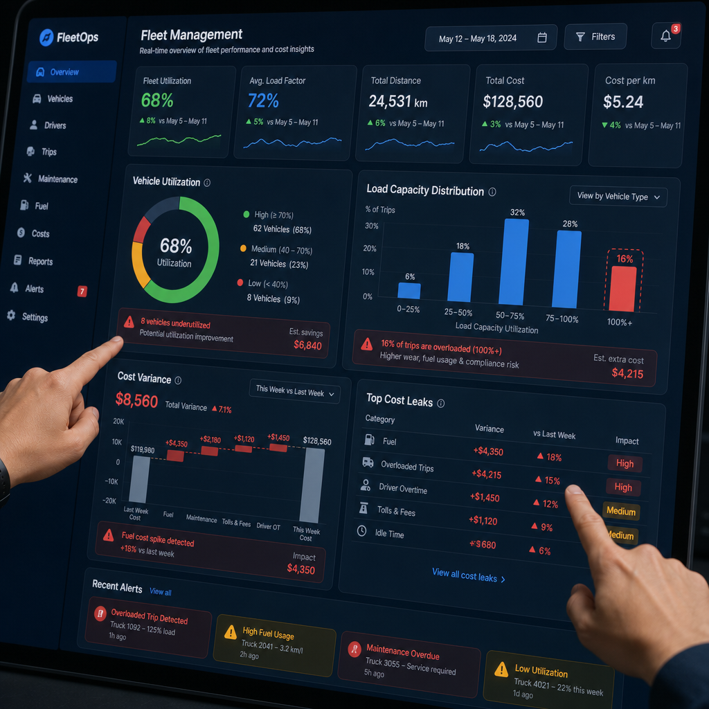
“The biggest operational savings we uncover are never in broken processes. They are in processes working perfectly as designed, where the design itself has become the liability.” Source: Flow Dynamics operational diagnostic findings across UK transport clients.
Pro tip: Before commissioning any system upgrade, spend five days capturing how your current planning decisions behave in live conditions. The gap between what the rules say and what the data shows is where your savings sit.
Rule 1: Fixed Route Assumptions Treated as Permanent
Fixed routes are a planning convenience that becomes a cost fixture. Operators assign consistent vehicle and driver combinations to recurring lanes because it simplifies scheduling. That is a reasonable starting point. The problem is when those routes are never re-examined against changes in demand density, fuel cost, or traffic pattern shifts that have occurred in the intervening years.
What the data reveals about static routing
When live hardware is deployed across a fleet running fixed routes, it consistently surfaces two problems. First, actual travel times and distances deviate materially from the planned route data embedded in the TMS. Second, vehicle capacity on fixed routes frequently runs at utilisation levels that would not be acceptable on dynamically planned routes, but because the route is fixed, nobody looks at the fill rate.
A common mistake is treating route fixed-ness as a service quality requirement when the customer contract does not actually require it. Many fixed routes exist because an ops manager preferred the predictability, not because the customer specified it. That preference costs real money.
For UK transport operators running between 20 and 100 vehicles, re-evaluating just the five highest-mileage fixed routes against current demand patterns routinely identifies £18,000 to £35,000 in annual savings from route consolidation alone, without changing service levels or customer commitments.
Rule 2: Fleet Sized to Peak Demand Rather Than Optimised Demand
This is the most expensive single decision rule in transport operations, and it is also the most defensible on the surface. Operations directors size fleet to cover peak periods because failing to meet demand at peak has immediate, visible consequences. The cost of carrying excess capacity during off-peak periods is diffuse, spread across depreciation, maintenance schedules, insurance, and driver hours, none of which appear as a single line item against the fleet sizing decision.
Calculating the real cost of peak-buffer vehicles
The calculation is straightforward once you run it. Take the number of vehicles that are utilised fewer than 60% of available operating days in a year. Multiply their combined annual total cost of ownership by the proportion of time they are sitting idle or running below viable utilisation. For a 50-vehicle fleet with eight vehicles in this category, that number routinely exceeds £140,000 per year when you include driver time attached to those vehicles on low-utilisation days.
The alternative is not simply disposing of assets. It is building demand-responsive allocation rules that allow the fleet core to absorb more of the demand range, and using spot or short-term subcontract arrangements for genuine peak events rather than maintaining permanent capacity for them. That structural shift requires changing the decision rule, not the vehicles.
Pro tip: Pull your vehicle utilisation data for the last 12 months and identify any asset used on fewer than 220 days. The annual cost of that vehicle almost certainly exceeds the cost of covering its demand through flexible subcontract arrangements on the occasions it would have been deployed.
Rule 3: Load Utilisation Thresholds Set Too Conservatively
Most transport operations run with a minimum dispatch threshold somewhere between 60% and 75% of load capacity. That threshold was almost certainly set based on a combination of customer SLA requirements and operational preference rather than a margin calculation tied to actual cost-per-unit-mile data.
The consequence is that operators frequently dispatch vehicles at 65% load when the marginal cost of filling the remaining capacity is near zero and the revenue or cost avoidance of doing so is material. Conversely, some operators run the threshold too low and dispatch part-loaded vehicles on lanes where consolidation would have been achievable with a modest scheduling adjustment.
Where the threshold logic breaks down
The threshold problem compounds because it interacts with route planning logic. A planning system told to dispatch when load reaches 70% will dispatch. It will not automatically check whether waiting 90 minutes would have allowed consolidation with a second load on the same lane, reducing the total vehicle count for that day by one. That check requires a decision rule that does not exist in most standard TMS configurations.
According to research from the UK Department for Transport, road freight vehicles in the UK run at an average load factor of around 67%, meaning a significant proportion of freight movement is operating below full potential efficiency. The operators sitting above 80% average load factor consistently show lower cost-per-tonne-kilometre and better transport savings outcomes without additional capital investment.

Rule 4: Driver Allocation Logic That Ignores Real Cost Variance
Driver allocation in most operations is managed on availability and compliance, meaning who is available, who has the right licence category, and who is within their hours. What it almost never accounts for is cost variance between drivers on the same route type.
In practice, fuel consumption variance between drivers on identical routes can range from 8% to 22% depending on driving style, route familiarity, and vehicle handling. At scale, that variance is not a training issue. It is a scheduling issue. Allocating high-consumption drivers to long-distance high-mileage routes while lower-consumption drivers run urban short-haul circuits compounds the cost difference unnecessarily.
Why this rule is almost never corrected
The reason this decision rule persists is that the data to expose it exists in telematics systems that are not connected to planning logic. Telematics tells you what happened. The allocation system makes decisions without consulting it. Those two systems rarely talk to each other in a way that would change the allocation rule in real time.
Correcting this does not require replacing either system. It requires identifying the allocation logic gap and building a bridge between the behavioural data and the scheduling decision. That intervention alone, on a 40-vehicle operation running significant motorway mileage, can recover between £12,000 and £25,000 in annual fuel cost through smarter route-to-driver matching.
Rule 5: Subcontractor Trigger Points Based on Outdated Cost Models
Every transport operation has a point at which it switches from running work in-house to subcontracting it out. That trigger point is usually expressed as a capacity threshold, a distance rule, or a lane-type classification. The problem is that the cost model underpinning that rule is almost always out of date.
Subcontractor rates in UK road freight have moved materially since 2020, driven by driver shortages, fuel surcharges, and rate renegotiations following the supply chain disruptions of that period. Meanwhile, the internal cost benchmarks many operators use to evaluate make-versus-buy decisions were last updated before those shifts occurred.
The compounding cost of early subcontract triggers
When the trigger fires too early, operators pay subcontractor margins on work they could have absorbed more cheaply internally. When the trigger fires too late, they absorb inefficient internal runs because the rule does not flag them as subcontract candidates. Both directions represent a logistics cost reduction opportunity that is invisible without current cost model data.
A common mistake is assuming that because subcontract rates have risen, the make decision now automatically wins. In some lane types that is true. In others, particularly for specialist vehicle requirements or time-definite urban delivery, current subcontractor pricing is still competitive against the true fully-loaded internal cost including driver overhead, vehicle depreciation, and admin burden. The decision needs current numbers, not inherited assumptions.
Rule 6: Dwell Time Tolerance Built Into Planning That Nobody Questions
Dwell time is the time a vehicle spends stationary at a collection or delivery point beyond the minimum required for the task. Every planning system absorbs some dwell time tolerance into route windows. The question is whether that tolerance reflects actual operational necessity or historical generosity that has calcified into a planning assumption.
In practice, dwell time tolerances are often set by operations planners who added buffer to avoid driver complaints about unrealistic schedules. That buffer then becomes a route design constraint that adds 15 to 30 minutes per stop across a full day’s routing. On a vehicle making eight stops per day, that is between two and four hours of hidden schedule inflation per vehicle per day.
How dwell tolerance hides its real cost
The insidious aspect of dwell time tolerance as a cost driver is that it never appears as a line item. It appears as route capacity. A vehicle that could theoretically run ten stops in a shift only routes for eight because the dwell buffer consumes the remaining window. That means either an additional vehicle is deployed or stops are deferred, neither of which shows up against the original dwell time decision.
For multi-drop urban operations, recalibrating dwell time tolerance to reflect actual measured dwell behaviour rather than planned buffer adds between one and two productive stops per vehicle per day on average routes. At scale across a 30-vehicle urban fleet, that is the equivalent of recovering between two and four full vehicle days of capacity weekly without adding assets or drivers.
Rule 7: Return Leg Planning That Defaults to Empty Miles
Empty running is the most visible transport inefficiency and also one of the most persistently unaddressed. According to the UK Department for Transport’s road freight statistics, approximately one in four heavy goods vehicle movements on UK roads runs empty. For operators with predictable outbound lanes, the return leg represents a structural opportunity that is regularly ignored because the planning system is not configured to look for it.
The decision rule at fault here is the one that treats the return leg as a scheduling residual rather than a plannable revenue or cost-recovery opportunity. Planning systems route vehicles outbound to specification and then simply route them home. The question of whether there is a backhaul opportunity on that lane is either handled manually, not handled at all, or delegated to a freight exchange that the planner checks inconsistently.
Building backhaul into planning logic rather than leaving it to manual effort
The fix is not a new system. It is a decision rule change. When planning logic is adjusted to flag return legs on routes above a defined mileage threshold as backhaul candidates before the route is locked, and when that flag triggers a defined check process rather than relying on planner discretion, backhaul utilisation rates increase materially.
For operators running consistent long-haul lanes, closing the backhaul gap from 25% utilisation on return legs to 55% utilisation represents a direct reduction in cost-per-kilometre that flows straight to margin. On a fleet covering 4 million kilometres per year with a meaningful proportion of long-haul activity, that single rule change is worth between £40,000 and £80,000 annually depending on lane mix and prevailing backhaul rates.
How These Rules Compare Across Different Operational Approaches
Not every approach to identifying and correcting decision rules delivers the same result. The method matters as much as the intention. Below is a direct comparison of three approaches operators commonly take when addressing fleet management decisions and transport operations cost.
| Approach | What It Uncovers | Limitations |
|---|---|---|
| Internal audit using existing TMS reports | Aggregated performance metrics, KPI trends, headline utilisation figures | Reports are built on the same planning assumptions causing the problem. They cannot surface what the rules are hiding. Decision-level cost variance remains invisible. |
| Consulting review using historical data | Pattern analysis across past 12 months, benchmark comparison against industry averages | Historical data reflects decisions already made. It shows outcomes, not the rule behaviour generating those outcomes in real time. Recommendations are often structural changes rather than specific decision corrections. |
| Live operational diagnostic with deployed hardware | Real-time decision behaviour, actual cost variance per rule, specific savings value by decision type | Requires five days of live deployment and operational access. Not suitable for operators unwilling to allow external visibility into live system behaviour. Findings are highly specific rather than general benchmarks. |
The live diagnostic approach is the one that consistently surfaces the largest and most actionable savings. The reason is straightforward: decision rules only reveal their true cost impact when you observe them operating on real loads, real routes, and real scheduling constraints, not when you model them against historical averages.
Pro tip: When evaluating any cost reduction engagement, ask the provider specifically how they identify decision-level cost variance rather than reporting-level inefficiency. If they cannot answer that question with a specific methodology, their findings will be limited to what your existing reports already show you.
Frequently Asked Questions
How do I know if my operation has decision rules that are costing significant money?
The most reliable indicator is a gap between your reported performance and your intuition about where costs should be. If your KPIs look acceptable but you cannot explain why margins are not improving despite volume growth, decision rules are almost certainly the cause. A second indicator is rules in your TMS or planning process that nobody can explain the original rationale for but that everyone treats as fixed constraints.
Do I need to replace my transport management system to fix these problems?
No. In the vast majority of cases, the rules generating the largest costs sit inside existing systems and can be changed without system replacement. The intervention is a rule modification, not a technology change. System replacement is expensive, disruptive, and rarely addresses the underlying decision logic problem because new systems get configured with the same inherited assumptions unless those assumptions are challenged first.
What is a realistic annual transport savings figure for a mid-sized UK fleet operator?
For a UK operator running between 20 and 80 vehicles across mixed route types, identifying and correcting the top three decision rules from this list typically produces between £80,000 and £250,000 in annual savings. The specific figure depends on current load utilisation rates, the proportion of empty running, and whether fleet sizing decisions have been revisited recently. Operations with higher fixed-route dependency and older cost models at the higher end of that range are common.
How long does it take to identify these cost-generating rules in a live operation?
With the right methodology and live system access, the primary decision rules generating material cost can be identified within five working days. This requires hardware deployed within the live operation rather than analysis of historical reports. The five-day window captures enough decision cycles across routing, dispatch, and allocation to identify statistically significant cost variance by rule type.
Are these problems specific to larger fleets or do smaller operators face the same issues?
The same seven decision rules appear consistently across fleet sizes from 15 vehicles upward. Smaller fleets often have more entrenched rules because there are fewer people in the planning function and less challenge to inherited logic. The absolute savings figure is proportionally lower on a smaller fleet, but as a percentage of transport operations cost it is often higher because there has been less scrutiny of the underlying assumptions.
Why do these decision rules persist if they are costing so much money?
Because they are invisible in standard reporting. A rule that adds unnecessary cost does not generate an alert. It generates a slightly worse KPI that gets attributed to fuel prices, driver availability, or customer demand patterns. Nobody goes looking for the decision rule as the cause because the reporting structure was not designed to surface it. The cost accumulates silently while the business optimises the variables it can see.
What decision rules are you currently running that have not been challenged in the last two years? Share your experience in the comments or reach out directly if you want to discuss what live diagnostics have surfaced in similar operations.
References
- UK Department for Transport road freight statistics and vehicle loading data
- McKinsey insights on logistics operations efficiency and cost reduction strategies
- Statista data on the UK logistics and transport industry performance metrics
- Forbes analysis of fleet management trends and transport cost optimisation
- UK Government overview of the logistics and supply chain sector including cost benchmarks