Your vehicle fill rates look acceptable. Your on-time delivery figures are holding steady. Your cost-per-kilometre hasn’t moved dramatically in the last quarter. So why does the overall transport budget keep climbing? The answer, in almost every operation we have worked with, is not in the metrics you are watching. It is in the space between them. Hidden transport costs accumulate not through obvious failures but through the slow compounding of flawed fleet allocation logic, outdated route assumptions, and planning rules that made sense three years ago but no longer reflect how the network actually operates.
Table of Contents
- Quick Takeaways
- Why Your KPIs Tell You Everything Except What’s Costing You Money
- The Hidden Utilisation Gap: What It Is and Why It Stays Hidden
- Fleet Allocation Logic: Where Cost Leaks Live and Breathe
- Route Assumptions That Have Outlived Their Usefulness
- What Proper Transport Operations Diagnostics Actually Looks Like
- Comparing Approaches to Transport Cost Reduction
- Fleet Utilisation Analysis: Moving from Averages to Decision-Level Data
- Frequently Asked Questions
- References
Quick Takeaways
| Key Insight | Explanation |
|---|---|
| KPIs measure averages, not decisions | Fleet fill rates and cost-per-mile figures smooth over the specific planning decisions where money is actually being lost. A 78% average utilisation rate can hide daily runs at 40% capacity. |
| The utilisation gap is a decision problem, not a data problem | Most operations already have the data. The issue is that planning rules and allocation logic were never designed to catch the gap between what vehicles carry and what they could carry. |
| Route assumptions age silently | Routes validated in 2019 are still being used in 2025 without review. Customer locations, delivery windows, and traffic patterns have changed. The planning rules haven’t. |
| Fleet allocation logic is the highest-impact lever for cost reduction | Which vehicle goes to which job, and when, is typically governed by rules set years ago. Correcting these rules alone frequently surfaces six-figure annual savings in mid-sized fleets. |
| Transport operations diagnostics must observe live behaviour | Analysing historical reports is not the same as observing how decisions are made in real time. Live observation reveals the gap between the plan and what actually happens on the ground. |
| System replacement is rarely necessary | The root cause of most hidden transport costs is logic and rules, not software. Fixing the decision-making layer produces savings without requiring new technology investment. |
| Five days of live data can be more valuable than months of reporting | A short, focused deployment of diagnostic hardware within a live operation captures the real cost behaviour that standard reports are designed to average out. |
Why Your KPIs Tell You Everything Except What’s Costing You Money
The fundamental problem with standard transport KPIs is that they are designed to show stability, not to surface loss. Vehicle utilisation percentages, cost-per-delivery figures, and on-time performance rates all report on outcomes averaged across the fleet and across time. They are useful for board reporting. They are almost useless for identifying where money is being wasted in specific planning decisions.
In practice, a fleet reporting 80% utilisation on paper might be running a significant proportion of its vehicles below 50% capacity on specific lane types, days of the week, or customer categories. The average conceals the outliers, and the outliers are where the cost lives. A common mistake is treating a stable KPI as evidence that the operation is optimised. It is not. It is evidence that nothing catastrophic has happened recently.
The data consistently shows that operations with the most entrenched hidden transport costs are often those with the most mature reporting systems. The better your dashboards look, the easier it is to miss the gap between reported performance and actual operational efficiency.
Pro tip: If your transport KPI dashboard has not triggered a major operational review in the last 18 months, that is not a sign that everything is working well. It is a sign that your metrics are not sensitive enough to detect the decisions that are costing you money.


The Hidden Utilisation Gap: What It Is and Why It Stays Hidden
The utilisation gap is the difference between what your vehicles are physically capable of carrying and what they actually carry when all planning decisions, scheduling constraints, and allocation rules are applied. It is not the same as empty running. A vehicle can be fully loaded on the outbound leg and running empty on the return, and your utilisation metric will tell you the operation is performing at 50%. The gap is more subtle than that.
Why aggregate metrics miss it
The gap hides in the granularity that aggregate reporting discards. When you look at weekly fleet utilisation, you lose the signal from Thursday afternoon runs that consistently leave at 55% capacity because the planning rule reserves space for late orders that rarely materialise. You lose the signal from a specific vehicle class being routinely dispatched for jobs that a smaller asset could handle at a third of the fuel cost.
According to McKinsey research on supply chain performance, the majority of logistics cost inefficiencies originate in planning and scheduling decisions rather than in execution. The execution is often fine. The problem is the plan the execution is following.
Why it compounds over time
Utilisation gaps do not stay static. Planning rules that produce a 10% inefficiency in year one tend to produce a 15% inefficiency in year three as the network changes and the rules are not updated. Every time a new customer is added, a new lane is opened, or a delivery window is shifted, the original logic that governed vehicle allocation becomes slightly less accurate. No one resets it. The gap widens.
“The biggest waste in freight and distribution is not fuel or labour. It is the cost of decisions made on assumptions that were never tested.” – Transport Economist, UK Freight Council Industry Review
Fleet Allocation Logic: Where Cost Leaks Live and Breathe
Fleet allocation logic refers to the rules, whether written into software or embedded in planner behaviour, that determine which vehicle goes to which job. This is the single highest-impact area for identifying hidden transport costs, and it is almost always the least examined.
How allocation rules become cost liabilities
Most allocation logic was set up when the fleet had a different composition, when customer requirements were different, or when the operation was running at a different volume. The rules made sense at the time. They were probably not documented in detail. Over time, planners learn to work around the rules rather than challenge them, because challenging allocation logic requires time and organisational energy that day-to-day operations do not allow.
The result is a set of allocation habits that no one owns, no one reviews, and no one can easily explain. In practice, this manifests as consistently sending a 7.5-tonne vehicle to a job that a 3.5-tonne vehicle could handle, or routing a vehicle through a depot consolidation step that adds 40 kilometres and serves no load-building purpose for that particular run.
The cost of a single bad allocation rule at scale
Consider a fleet of 30 vehicles where an allocation rule causes an unnecessarily large vehicle to be dispatched on a specific lane type twice per week. If the cost difference between the appropriate and allocated vehicle is £85 per run, that single rule costs approximately £8,800 per year. Most operations have multiple such rules. The annual exposure across a mid-sized fleet is routinely in six figures. This is the territory that Flow Dynamics is specifically built to identify, using live observation rather than retrospective reporting.
Pro tip: Ask your planning team to explain the last five vehicle allocation decisions they made without referring to software outputs. If they cannot articulate the logic clearly, the decisions are being driven by habit rather than optimised rules, and that habit is costing you money.
Route Assumptions That Have Outlived Their Usefulness
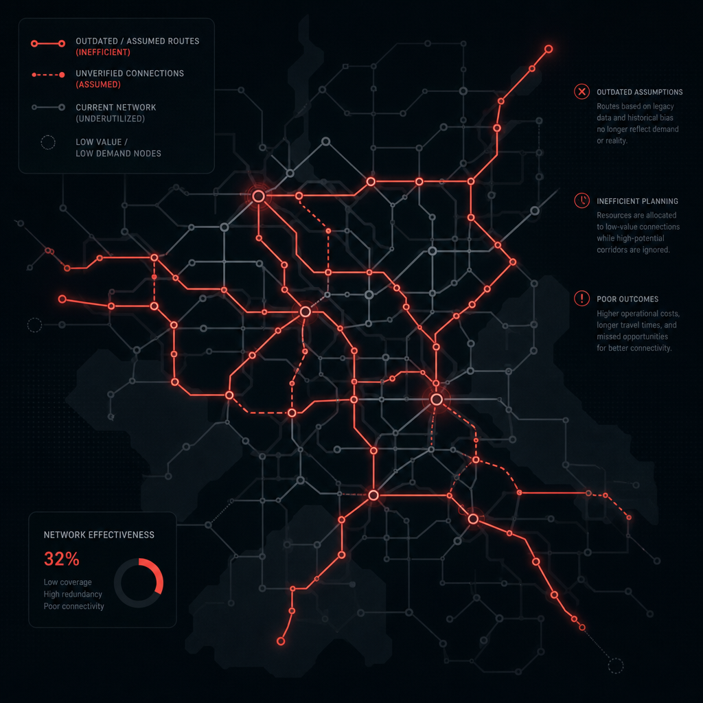
Route assumptions are the specific beliefs baked into planning about how a particular lane, customer stop, or delivery sequence should work. They include assumptions about travel time, loading sequence, delivery window compliance, and vehicle suitability. They also include the quieter assumptions: that a particular depot is the right consolidation point, that a certain day is the best day to serve a cluster of customers, or that a specific driver sequence minimises mileage.
These assumptions are often years old. They were validated, if they were validated at all, in a different operating environment. Customer bases have shifted geographically. Delivery windows have tightened or changed. Traffic patterns have altered. New distribution points have opened. The assumptions have not been revisited.
How outdated route assumptions inflate cost invisibly
The insidious quality of an outdated route assumption is that it does not produce obvious errors. The vehicle leaves on time, delivers on time, and returns to base. The cost-per-delivery figure looks reasonable because it is being compared to the same route from last year, which was also based on the same outdated assumption. There is no baseline of what the route should cost if it were designed from current conditions.
A route that could serve eight customer stops in a single efficient loop might instead be running as two sequential routes because an assumption about delivery window incompatibility was never tested against the customers’ current operating hours. The extra vehicle movement, extra driver shift, and additional fuel cost are all invisible in standard reporting because the reporting compares actual against plan, not actual against optimal.
What Proper Transport Operations Diagnostics Actually Looks Like
Most transport consultancy approaches to cost reduction fall into one of two categories: either they analyse historical data and produce a report, or they recommend a new technology platform and call that optimisation. Neither approach reaches the actual problem.
Analysing historical data tells you what happened on average. It does not tell you why specific planning decisions were made in real time or how planner behaviour differs from the documented process. A report based on three months of historical fleet data will identify trends. It will not identify the allocation habit that a specific planner follows every Tuesday morning because it was how they were trained in 2018.
Why live observation changes everything
Proper transport operations diagnostics requires observing decision-making as it happens. This means being present in the planning environment, watching how vehicles are allocated to jobs in real time, tracking how routes are adjusted during the day, and capturing the gap between the planned operation and the executed operation. This is precisely what Flow Dynamics does with its proprietary hardware deployed within live systems over a five-day window.
Five days is sufficient because the patterns that generate cost leaks are consistent. An allocation rule that causes unnecessary cost on a Monday will cause it every Monday. A route assumption that adds unnecessary kilometres does so on every run. Live observation over five working days captures the full weekly pattern of decisions and surfaces the specific points where cost is being generated.
What diagnostics must not do
Diagnostics that focus purely on reporting metrics miss the decision layer entirely. If your transport operations diagnostic process produces a new dashboard without identifying specific planning decisions to change, it has not found the problem. The goal is not better visibility of the same inefficiencies. The goal is identifying which decisions need to change and by how much that change will reduce cost.
Comparing Approaches to Transport Cost Reduction
| Approach | What It Examines | Limitation for Hidden Cost Identification |
|---|---|---|
| Retrospective Data Analysis (e.g., standard consultancy reports) | Historical KPI trends, cost-per-route averages, fleet utilisation aggregates over 3-12 months | Averages mask the specific decision-level inefficiencies where cost accumulates. Cannot capture real-time planning behaviour or the gap between documented process and actual planner decisions. |
| New Technology Platforms (e.g., TMS or route optimisation software vendors) | Route optimisation algorithms, scheduling automation, digital workflow replacement | Addresses output optimisation but does not audit the allocation logic and planning assumptions being fed into the system. Automating a flawed decision rule makes it more consistent, not more efficient. |
| Live Operational Diagnostics (e.g., Flow Dynamics methodology) | Real-time planning decisions, allocation logic in practice, route assumption validation against current conditions, vehicle deployment patterns during a live five-day window | Requires physical deployment within the operation. Cannot be delivered entirely remotely. The tradeoff is that it surfaces the specific, actionable decisions that retrospective analysis and software implementation both miss. |
Fleet Utilisation Analysis: Moving from Averages to Decision-Level Data
Standard fleet utilisation analysis reports on what percentage of available capacity was used across the fleet over a defined period. This is useful for high-level performance tracking. It is not useful for identifying where and why specific vehicles are being underused, because it does not connect utilisation figures to the planning decisions that produced them.
Decision-level utilisation analysis asks different questions. Not “what was our average utilisation this month?” but “which allocation rule caused vehicle 14 to run at 52% capacity on the same lane type every Thursday, and what would utilisation look like if that rule were corrected?” The second question is harder to answer with standard reporting tools because it requires connecting vehicle behaviour data to the specific planning logic that drove it.
The difference between load fill and effective utilisation
Load fill is the ratio of cargo weight or volume to vehicle capacity on a given run. Effective utilisation is a broader measure that accounts for whether the right vehicle was deployed for the job, whether the route served the maximum logical number of stops given current customer locations, and whether the scheduling sequence minimised idle time and empty running. A vehicle can have a high load fill and still represent poor effective utilisation if it is the wrong vehicle class for the job.
Operations that track load fill and call it utilisation analysis are missing the second and third layers of the problem. This is why transport cost reduction efforts that focus on improving load fill percentages often plateau. They address one dimension of the problem while leaving the others untouched.
What decision-level analysis reveals in practice
In practice, decision-level fleet utilisation analysis consistently reveals three types of cost leak. First, systematic over-specification of vehicle type for certain job categories, driven by allocation rules that default to larger assets when smaller ones would suffice. Second, route sequencing that prioritises planner convenience or historical habit over mileage efficiency. Third, scheduling patterns that create vehicle availability gaps, forcing the use of suboptimal assets on runs where the preferred asset class is already committed.
Each of these is a decision problem, not a reporting problem. Fixing the decision corrects the cost. Adding better reporting about the same flawed decision does not.
Pro tip: When running a fleet utilisation analysis, segment your data by vehicle class, lane type, day of week, and planner. If you find that utilisation varies significantly by planner on identical lane types, the allocation logic is not being applied consistently, and the inconsistency is producing unnecessary cost on the lower-performing side.
Frequently Asked Questions
What are hidden transport costs and how are they different from visible operational costs?
Hidden transport costs are the expenses generated by flawed planning decisions, outdated route assumptions, and inefficient fleet allocation logic that do not appear as obvious line items in your cost reporting. They are embedded in the cost of running the operation as planned, rather than appearing as variances or overruns. Because they are baked into normal operations, they look like baseline cost rather than waste. Visible costs, by contrast, are things like fuel surcharges, breakdown repair, or overtime payments that appear as discrete budget items and trigger direct management attention.
Why does transport cost keep rising even when KPIs appear stable?
Stable KPIs reflect averages across the fleet and across time. They do not reflect whether the underlying planning decisions are optimised. As a network evolves, customer requirements change, and fleet composition shifts, the original planning rules that generate those averages become progressively less efficient. The cost rises because the rules are producing more waste per run than they used to, but the KPI averages smooth over that deterioration. The gap between actual cost and optimal cost widens, while the reported metrics remain within acceptable ranges.
How long does it take to identify hidden transport costs in a live operation?
A focused diagnostic deployment across a live operation over five working days is sufficient to identify the primary cost leaks in most mid-to-large fleets. This is because the planning decisions and allocation habits that generate cost are consistent. They follow the same patterns week to week. Five days captures a full operating cycle including the weekly scheduling rhythm and the specific decision points where planner behaviour diverges from optimal allocation logic. Longer observation periods add breadth but rarely change the primary findings.
Is fleet allocation logic the same as route optimisation?
No, and conflating the two is one of the most common mistakes in transport cost reduction programmes. Route optimisation refers to finding the most efficient sequence and path for a vehicle to service a set of stops. Fleet allocation logic refers to the rules that determine which vehicle is assigned to which job before any routing takes place. You can have a perfectly optimised route being run by the wrong vehicle type, which means the route optimisation is correct but the cost is still higher than necessary. Both layers need to be examined independently.
Do you need to replace your TMS or fleet software to fix hidden transport costs?
No. In the vast majority of cases, the root cause of hidden transport costs is the logic and assumptions being applied within the existing system, not a deficiency in the system itself. Replacing a TMS while retaining the same allocation rules and route assumptions will reproduce the same cost leaks in the new platform. The fix is to correct the decision layer, the specific rules, assumptions, and planning habits that drive how the system is used. System replacement is a significant investment that addresses the wrong problem if the underlying decisions are not fixed first.
What is a realistic scale of savings from addressing hidden transport costs?
For mid-sized fleets operating 20 or more vehicles across regular lanes, annual savings from correcting fleet allocation logic and route assumptions typically fall between £100,000 and £400,000, depending on fleet size, lane complexity, and how long the underlying inefficiencies have been in place. The savings scale with the size of the operation and the age of the planning rules. Operations that have not reviewed their allocation logic in three or more years consistently show the largest gaps between current and optimal cost.
What is your experience with transport KPIs that looked healthy on paper while actual costs continued to climb? We would be interested to hear what you found when you looked more closely at the planning decisions behind the numbers.
References
- McKinsey and Company: Research and insights on supply chain efficiency, logistics cost structures, and operational performance improvement
- Statista: Statistical data on UK and European transport and logistics operating costs, fleet management benchmarks, and freight market trends
- Forbes: Business analysis and executive perspectives on operational cost management and supply chain decision-making
- UK Government: Department for Transport publications on freight efficiency, fleet emissions standards, and transport network performance data
- Ahrefs Blog: Data-driven content and industry analysis methodology referenced for benchmarking performance gap analysis approaches